Astronomy - Online Labs
Compare photos to maps of the constellations.
On star maps, you see only the brightest stars of a constellation.
This is deceiving, because the stars might be rather faint in reality -
e.g. Ophiuchus and Ursa Minor, or smaller than you think - Triangulum and
Delphinus. Therefore you should become familiar with the constellations
how they really look like in a sky with little light pollution.
The photos are not labeled, but instead lettered from A to S.
Procedure:
| C O N S T E L L A T I O N S | |
|---|---|
| (Her, Cas, Crv, And, Leo) | (Sco, UMi, Ser, Vir, Oph) |
| (Lib, Ori, Peg, Per, Aql & Del) | (Cyg, Cep, CMa & CMi, Boo & CrB) |
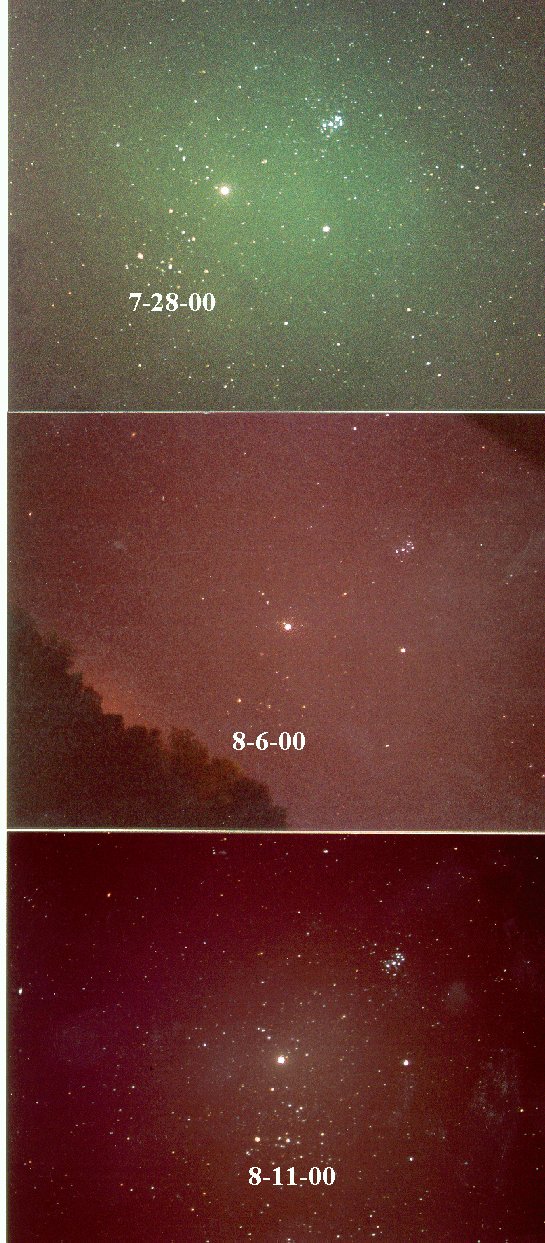
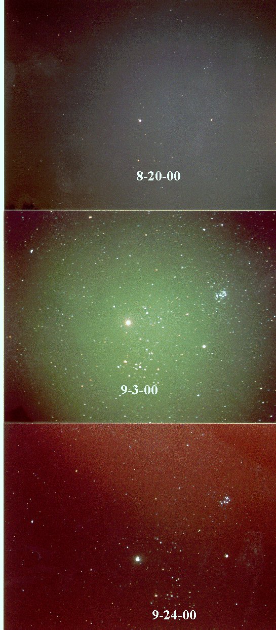
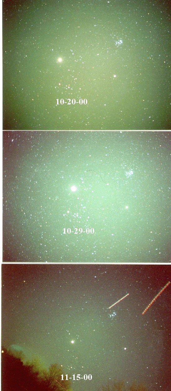
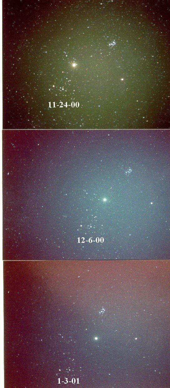
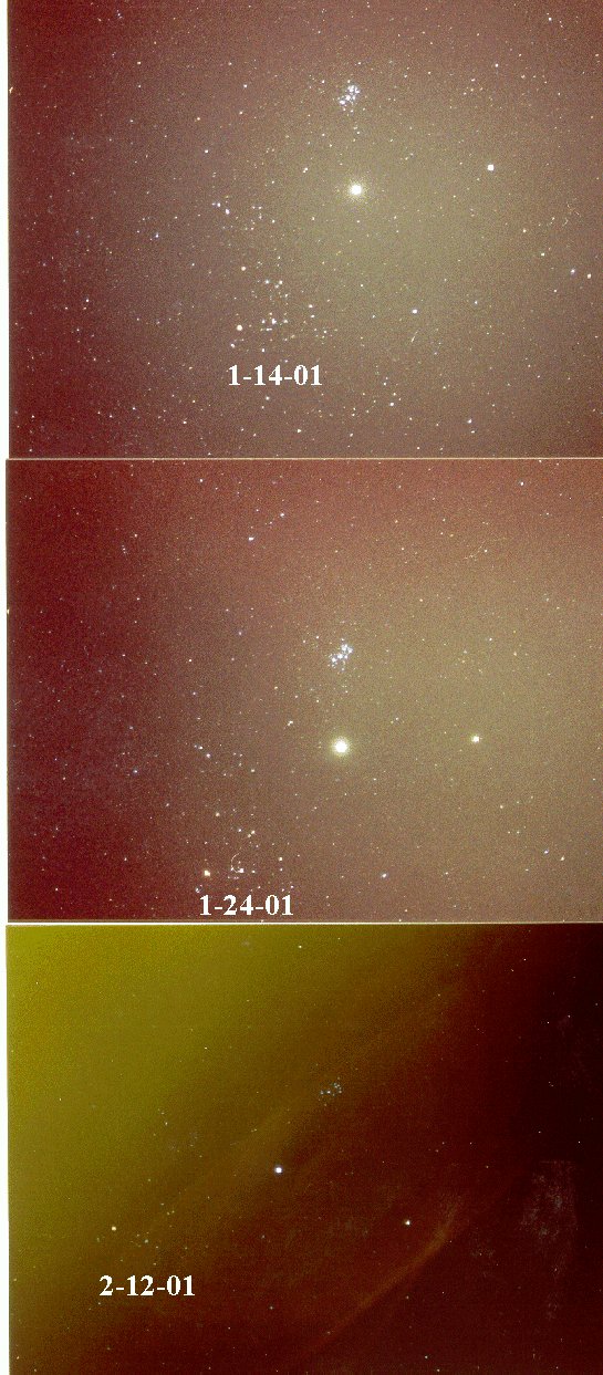
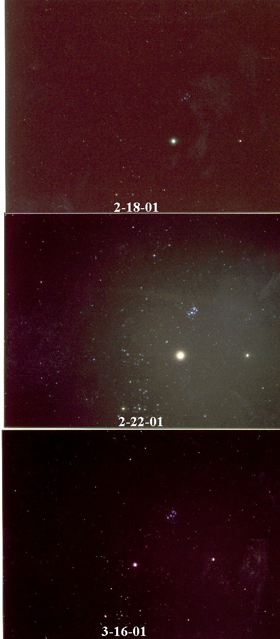
Objective: This lab shows that (a) planet(s) "wander"(s) across the sky (the sky-background is comprised of the stars), whose motion is apparent over the course of some weeks/months. Stars, however, have always the same positions with respect to each other (excluding Earth's parallax and precession and the star's proper motion, which are of no concern to casual observing as we do it).
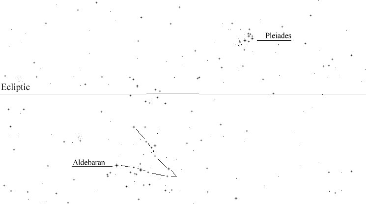
Planets: Jupiter and Saturn (for summer 2000 until spring 2001), Jupiter (for fall 96), Mars (for spring, summer and fall 97). This lab usually done for Jupiter in Taurus in 2000/01 only.
When comparing the light of planets with that of stars, what is an obvious difference? How is this difference produced?
Note: please do not print the photos! It would be a waste of
ink and the resulting print will be terrible anyway. Do these online labs
with the pictures on the screen.
| July_28,_Aug_6, 11 | Aug_20,_Sep_3, 24 | Oct_20, 29,_Nov_15 | Nov_24,_Dec_6,_Jan_3 |
| Jan_14, 24,_Feb_12 | Feb_18, 22,_March_16 |
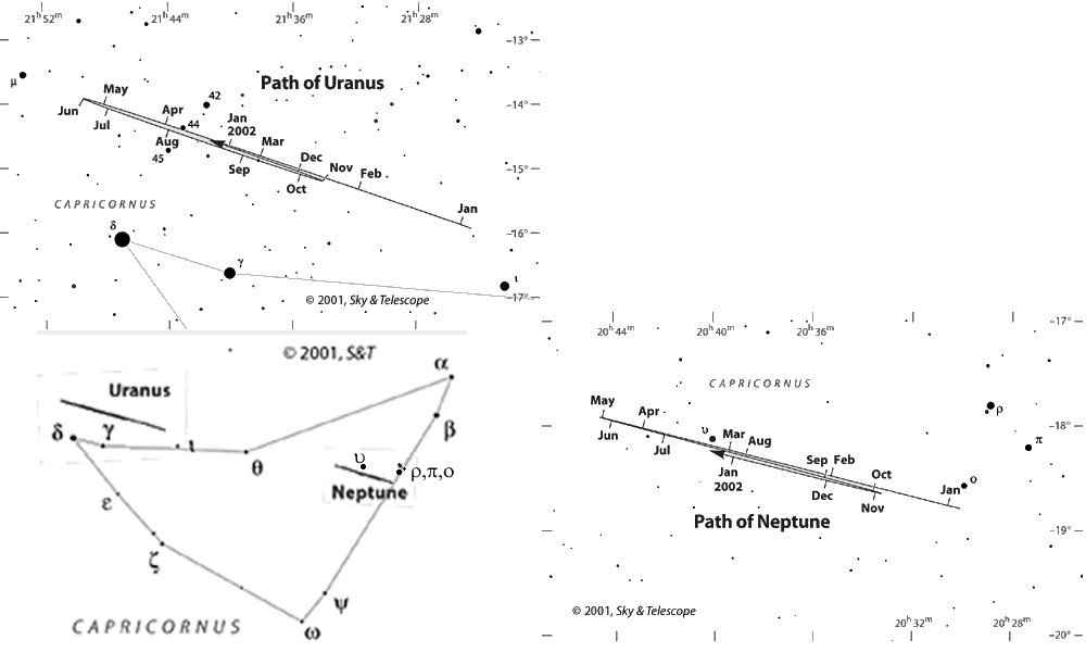
Procedures (also applicable to Mars, Venus, Uranus):
| J U P I T E R | ||
|---|---|---|
| May - Aug 96 | Aug - Nov 96 | November 96 |
| M A R S | ||||
|---|---|---|---|---|
| Aug - Sep 96 | Nov 96 - Jan 97 | February 97 | March 97 | March 97 |
| April 97 | May 97 | June 97 | July 97 | August 97 |
| September 97 | October 97 | |||
You can check your results for Mars' motion using Nick
Strobel's diagram of Mars' motion from November 96 to August 97.
Venus (Aug
- Oct 96)
Venus
(November 96)
Uranus is moving very slowly and is pretty faint, so photos are blow-ups, ...
0.4 m Gettysburg College Observatory
The latter two are at Kitt Peak National Observatories (20 miles west of Tucson, AZ).
Watch the explanations on video which is supplied at each center in Alliance, Sidney and Scottsbluff.
CLEA (Contemporary Lab Exercises in Astronomy - Gettysburg College, PA, and National Science Foundation) provides several computer labs for students. Two of them let you analyze starlight.
With Photometry you determine the apparent brightness of stars, with Stellar Spectra you determine their spectral type.
CLEA provides the starfield of the Pleiades cluster, for which plenty of information is already available, most importantly an HR-diagram with data from former students.
All stars in the Pleiades are at approximately the same distance (give or take a few lightyears - insignificant at 400 lightyears) from our solar system. This assumption is justified for several reasons. First, they are all clustered, i.e. lots of fairly bright stars in a very small region. Second, positional measurements over years showed that they all move towards the same vantage point (we won't do this exercise - too little time). Third, the labs that you do will show that all stars lie on a line (the Main Sequence) in the HR-diagram - even by plotting apparent magnitude on the y-axis - another very good indication for the same distance. Fourth, all open clusters (and of course globular clusters) show similar patterns in their HR-diagrams when plotting apparent magnitude. Fifth, these nice patterns also strongly suggest that stars in a cluster formed at the same time. If that wasn't the case (i.e. not same distance nor same age) we'd find stars scattered all over the HR-diagram. But we don't ... so the assumptions same distance and same age must be correct.
Photometry gives you the apparent brightness. With the HR-diagram (and another calibrated one, e.g. Hipparcos), you'll be able to determine the Pleiades' absolute brightness and with these two, you get the distance (fairly accurate). We are also able to determine the age of the Pleiades (ballpark figure).
We also determine the star's color index B-V, i.e. by how much the brightnesses in the Blue and Visual (yellow) differ, which gives us the spectral type as well (see last table in my Stellar Evolution Appendix).
Stellar Spectra gives you the spectral type as well (B-V and spectral analysis should confirm each other). This in turn - with your knowledge about absorption lines - reveals a star's surface temperature (see first table in my Stellar Evolution Appendix), and perhaps a Doppler-shift, rate of star rotation, strength of magnetic field, chemical composition of its atmosphere (these we won't do).
Surface temperature and absolute brightness give us the size (radius) of each star (Stefan-Boltzmann law). The luminosity-mass relationship (for main sequence stars only) give us a star's mass.
And a good astrophysics book on stellar structure and evolution (e.g. by R. Kippenhahn and A. Weigert) would give us the star's structure, core temperature, mode of nuclear fusion, life expectancy, evolution, etc. etc.
Some definitions:
Color index B-V is the brightness comparison between Blue and Visual (yellow):
(mB - mV) = - 2.5 log ( count_B / count_V ) .
Apparent magnitude m is the apparent brightness (as seen from Earth) measured in magnitudes:
Magnitude-Brightness relation (m1 - m2) = - 2.5 log ( count_1 / count_2 ) , compared to another star (that's Alcyone in our case).
HR-diagram , i.e. Hertzsprung-Russell diagram, plots absolute
magnitude versus temperature (or color index, or spectral type).
In our case, we plot apparent magnitude versus color index.
Procedure:
Do this together (2 or 3 people)!!! It'll make this
much easier.
Access CLEA's Classification of Stellar Spectra.
- Log In (initial is fine)
- Run Take Spectra
- Click Dome to
open it
- Click Tracking , so
that the telescope follows the star's apparent movement
- these are not the Pleiades, so click on Field
and choose the Pleiades
- Later on you will take data of a faint star. You may want to use a telescope with a larger aperture. So click on Telescopes, Request Time, then 4.0 m Mayall. Most likely you won't get it (but it's worth a shot). Then try Telescopes, Request Time, then 1.0 m KPNO. If you're lucky, click on Telescopes, Access ...
- Play a little around
- Click and hold down on E, N, W, or
S
- click on slew rate and it changes from
4 to 8, 16, 1, 2, back to 4, with that you move faster or slower across
your starfield
- Do a test on Electra (type in its coordinates:
3h 41m 56s, 23d 57' 55"), the second brightest star.
- Center Electra in the red rectangle, which shows
you the size of the monitor
- Click on Monitor
- Move Electra in between the red vertical bars
- Take Reading, click on Start/Resume
Count
- After a short time (10 - 20 sec.) you notice
that the spectrum doesn't change its shape anymore (if you get totally
useless information, you probably haven't put the star in between
the lines - so Return (do not save)
- Stop Count
- Save as Ele
(- write down Electra's HD number)
- Note that the spectrometer measures between
3900 Å and 4500 Å, i.e. in the far-violet part of the spectrum
only
- Return (write down the coordinates)
and Run , then Classify Spectra
- Load Unknown
Spectrum Saved Spectra (*.CSP)
Electra's spectrum
- Config Display
Grayscale "Photo"
- Load Atlas
of Standard Spectra Main Sequence
(minimize
this MS window to keep the screen from overcrowding)
- Now you can analyze Electra's spectrum
- You can Load
Spectral Line Table (but don't have to - notice that your
screen gets crowded)
- click and hold while moving around in the spectrum
shows you which elements produce spectral lines --- compare to spectral
line diagrams in your book (after playing with that, minimize this Spectral
Line Identification window)
- Click Down (or
Up)
and compare your spectrum (in the middle) with the main sequence spectra
- change back to Config
Display Intensity Trace , which works better
because now you can click on Difference : the
closer the wiggly red line is to a horizontal the better is the match.
- determine Electra's spectral type
- I determined B 2
Also, write down Electra's HD # as the star's name (HD
# should appear during measurement and classification).
Access CLEA's Photometry.
- Log In (initial is fine)
- Start
- Click Dome to
open it (you see the Pleiades)
- Click Tracking , so that the
telescope follows the stars' apparent movement
- Continue the test on Electra
- Find and center Electra in the red rectangle
(or use its coordinates), which shows you the size of the monitor
- Click on Monitor
- Move Electra into the red circle
(the size of the photometer)
- Note that the Filter
is set on V (visual, which measures primarily
yellow)
- Click on Take Reading
, which automatically takes 3 readings for 10 sec. each (therefore you
wait for 30 seconds). Take reading means that the photometer counts
the number of photons received from Electra.
- Write down Mean/Sec
, which is the average # of photons per sec. (not per 10 sec.)
- Compare this result to V = 2,600,000 (my reading
from 3-13-97)
- Change the Filter
to B (blue)
- Take Reading , write down Mean/Sec
, compare to B = 2,877,000 (A. Veh, 3-13-97)
Do not do the following on your own as I don't want you get frustrated.
Leave this analysis to me.
- use the color index B-V relation to determine
(mB - mV) and compare to my (mB - mV) = - 0.11 mag
- with your B-V and (see Lecture notes, Stellar
Evolution, Appendix) determine Spectral Type and Surface Temperature
- compare to my results B 8 and T = 12,000
K
- use Electra's and Alcyone's V-counts and the
Magnitude-Brightness relation to determine the magnitude difference (m1
- m2)
- with Electra's V1 = 2,600,000 and Alcyone's V2
= 5,636,000 you get (m1 - m2) = 0.8 mag- add this to Alcyone's mV = 3.0
mag and you get an apparent magnitude of mV = 3.8 mag for Electra
End of "do not do this on you own."
Now that you're familiar with this software, here are your actual measurements.
- toggle back to Stellar Spectra
- get Back to the telescope
window (you need to leave the classification window)
- get the telescope view of all of the Pleiades (maybe
you need to leave Monitor ).
- choose a fairly faint star (the bright stars are
most likely taken up) !
- Take Reading , then click on Start/Resume
Count
- after a short while, the pattern of the spectrum will
become apparent - time to stop. If this is not happening, it means
that the signal/noise ratio is very low, and you better get a larger telescope
or move to a slightly brighter star than this one.
- follow the above steps (the ones you did for Electra),
take spectrum, classify, measure its V and B in photometry
- don't forget to write down the coordinates as well
After that turn in your work. Your data will add one more star to this HR-diagram (April 12, 1998).
Here is a routine for the TI-83 to graph the UBV data, fit a Black-Body curve to it and determine the correct temperature.
3STO>dim(LIN)
{365,440,550}STO>LNM
6.26E-34STO>H:1.38E-23STO>B:3E-8STO>C
For(J,1,3)
Disp "UBV":Input U:USTO>LIN(J)
End
LIN/LIN(3)STO>LIN
Repeat 5>7
Disp "TEMPERATURE":Input T
550^3.5*(e^(H*C/550*10^(9)/(B*T))-1)STO>K
"K/X^3.5/(e^(H*C/X*10^(9)/(B*T))-1)"STO>Y1
DispGraph:Pause :End
Documentation: execute the routine; exit it right away (this was just for defining the lists IN and NM [intensity and nanometers]); insert these lists as x and y in a StatPlot; change the window settings to x: 200, 700 and y: 0, 2 ; now start the routine; it asks you for UBV three times (type in the measured UBV from CLEA photometry in that order); the three data are scaled, so that LIN(3)="V"=1 all the time and the V datapoint will also always appear on the Black-Body curve; supply an estimated temperature; the curve and data are plotted and you judge how good the curve; hit enter to try a new temperature (you're in an endless loop - exit with ON).
PS My exponent for the wavelength in the Planck curve is 3.5 because that fits most data (in order to achieve the correct temperature when checking the B-V in a table).
| DATE | t [min] | Df [Hz] | sep. [deg] | R [mill. km] |
| February 20 | 23.0 | - 6,300 | 2.4 | 60 |
| March 13 | 17.9 | + 101,000 | 14.9 | 46 |
| April 10 | 9.7 | - 28,300 | 7.4 | 64 |
| April 28 | 12.4 | - 91,400 | 26.9 | 70 |
| May 22 | 18.8 | - 93,500 | 20.3 | 57 |
| June 10 | 21.9 | + 2,600 | 1.1 | 46 |
A radar beam is sent out from Earth which is reflected and then after
some time t [min] received on Earth. Due
to the moving Mercury, the frequency f = 430 MHz
is Doppler-shifted by Df [Hz].
The line-of-sight velocity vo is determined via
the appropriate Doppler-equation: vo = ( Df
/ 2 f ) c with the speed of light c = 300,000 km/s.
The orbital velocity is obtained using the geometry of Mercury's orbit
with respect to Earth. For a very good account see Hoff ...
Only the equations shall suffice here.
Lab K4 Proper Motion of Barnard's star
All images are from the above website. Hipparcos was a satellite launched by ESA (European Space Agency). It made the most precise astrometric measurements (position and distance) of 100,000 stars and their proper motion (perpendicular to our line of sight; in contrast, radial velocity along our line of sight is determined via the Doppler effect - but Hipparcos had no spectroscopic objectives).
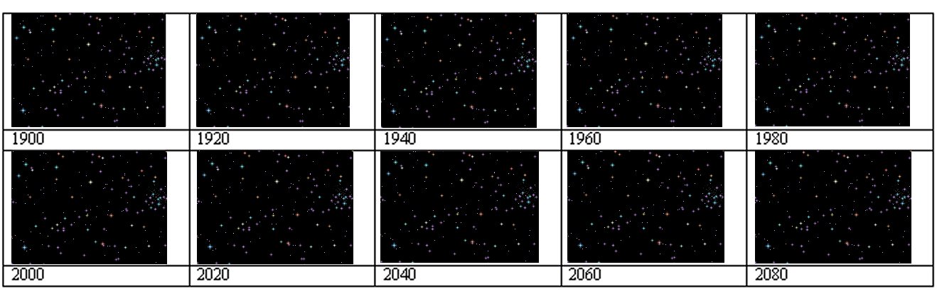
Objective: Determine how fast Barnard's star moves.
Determine (measure, estimate and calculate) how many degrees Barnard's
star moves per year. The six images are 20 years apart, starting
with the year 2000, ending with 2100. During this time frame the
other stars stay put. The coordinates of the star on the bottom are
R.A.=175822 and Dec.=+035709 , the star at the upper right has R.A.=175605
and Dec.=+051017 . (Coordinates are in (+degrees) hours, (arc)minutes,
(arc)seconds, each has two digits.)
When done compare this star field from the next century to the year
14000 (Barnard's star is long gone).
Of course, you can do the whole thing quicker by accessing ESA's
Hipparcos website and extracting the coordinates of Barnard's star
directly.
Determine the ages of the following star clusters by
| M5 at SEDS
A globular cluster in Serpens Caput, easily observable with binoculars (5.7 mag). |
M44
at WEBDA
The Beehive or Praesepe, an open cluster, the most obvious object in Cancer (naked eye; 3.6 mag). |
The Messier Object
Index at SEDS. I found the above HR diagrams by accessing this
web site first.
After reading your textbook and my "Measuring Stars" script, reason why the turn-off point gives the age of a star cluster.